Version 1.0, updated 2022-02-04

So, we have the data that we want to process uploaded to GPU memory. We have the shader module that is supposed to process the data precompiled and ready to use (at least technically). We have the logical device configured with a compute queue that would be able to run the processing commands. The problem is: none of these building blocks know anything about one another yet. The queue has no idea that it is supposed to run our shader module, and the shader has no idea where to find the data to process. We somehow need to bring those building blocks together. For that purpose we need to create a pipeline.

Pipelines

A pipeline object represents the configuration of the whole processing chain on the GPU. This includes the layout of the different stages and how the data flows between them, as well as the concrete shaders that are to be used in the various stages and the layout of the data itself.Graphics pipelines can get very very complex, with multiple shader stages and additional graphics functionality like blending modes, backface culling, primitive topology etc. plus all the associated data. Fortunately for us compute pipelines are much simpler as they essentially only have one stage: the compute shader stage.

Pipelines are created via the logical device. There are dedicated functions for each type of pipeline:

class Device
{
    ...
    // return values are actually ResultValue< UniquePipeline >, see chapter 2
    UniquePipeline createGraphicsPipelineUnique( PipelineCache pipelineCache, const GraphicsPipelineCreateInfo& createInfo, ... );  
    UniquePipeline createComputePipelineUnique( PipelineCache pipelineCache, const ComputePipelineCreateInfo& createInfo, ... );
    UniquePipeline createRayTracingPipelineKHRUnique( ... );
    ...
};

So we need two parameters for our compute pipeline. The PipelineCache is a helper object that can be used to speed up pipeline (re-)creation. It is recommended to use, but you can also pass in a temporary object. That’s what we will do in this tutorial. The ComputePipelineCreateInfo looks like this:

struct ComputePipelineCreateInfo
{
    ...
    ComputePipelineCreateInfo& setFlags( vk::PipelineCreateFlags flags_ );
    ComputePipelineCreateInfo& setStage( const vk::PipelineShaderStageCreateInfo& stage_ );
    ComputePipelineCreateInfo& setLayout( vk::PipelineLayout layout_ );
    ComputePipelineCreateInfo& setBasePipelineHandle( vk::Pipeline basePipelineHandle_ );
    ComputePipelineCreateInfo& setBasePipelineIndex( int32_t basePipelineIndex_ );
    ...
};

There is quite a number of flag bits we could set as the PipelineCreateFlags, but none of them are really relevant for us at this point. The functions related to the BasePipeline come into play when you want to derive one pipeline from another one (a bit like class inheritance in C++). We’re not going to need that here either. Which leaves two functions that we need to look at: setStage and setLayout.

The Compute Shader Stage

As said, compute pipelines are pretty straightforward in that they only have the compute stage. How that stage is to be configured concretely is determined by a PipelineShaderStageCreateInfo structure which looks like this:

struct PipelineShaderStageCreateInfo
{
    ...    
    PipelineShaderStageCreateInfo& setFlags( vk::PipelineShaderStageCreateFlags flags_ );
    PipelineShaderStageCreateInfo& setStage( vk::ShaderStageFlagBits stage_ );
    PipelineShaderStageCreateInfo& setModule( vk::ShaderModule module_ );
    PipelineShaderStageCreateInfo& setPName( const char* pName_ );
    PipelineShaderStageCreateInfo& setPSpecializationInfo( const vk::SpecializationInfo* pSpecializationInfo_ ) ;
    ...
};

That’s quite a few potentially relevant fields, let’s look at them one by one:

• once more, although there are some PipelineShaderStageCreateFlagBits specified, we can ignore the flags_ parameter for our usecase.
• the stage_ parameter determines the stage in the pipeline that this create info configures. For us that is obviously ShaderStageFlagBits::eCompute
• module_ is the shader module we created in the last lesson.
• setPName is used to specify the entry point into the shader, i.e. the name of the top-level function to call for this shader stage. That makes sense because SPIR-V allows for multiple entry points in one shader. However, multiple entry points are to my knowledge not yet supported by GLSL, so creating such a shader module would be more involved than simply compiling GLSL code. We’ll therefore stick to main as our shader entry point.
• SpecializationInfo can be used to configure so-called specialization constants. That’s a mechanism that allows for configuring a shader at pipeline creation time, e.g. for configuring the local workgroup size according to the device’s capabilities. We won’t use this feature, so we’ll ignore also this function.

That means we can create our PipelineShaderStageCreateInfo like so:

const auto shaderStageInfo = vk::PipelineShaderStageCreateInfo{}
    .setStage( vk::ShaderStageFlagBits::eCompute )
    .setPName( "main" )
    .setModule( *computeShader );

That wasn’t too hard, was it? With that our pipeline would know already which shader to use.

Pipeline Layout

Let’s now look at the second structure that we need to create our pipeline, the PipelineLayout. That one represents the configuration of the pipeline in terms of how the data that is processed in the pipeline is structured. It is created using the familiar pattern:

class Device
{
    ...
    UniquePipelineLayout createPipelineLayoutUnique( const vk::PipelineLayoutCreateInfo& , ... );
    ...
};

… with:

struct PipelineLayoutCreateInfo
{
    ...
    PipelineLayoutCreateInfo & setFlags( vk::PipelineLayoutCreateFlags flags_ );
    PipelineLayoutCreateInfo & setSetLayouts( const container_t< const vk::DescriptorSetLayout >& setLayouts_ );
    PipelineLayoutCreateInfo & setPushConstantRanges( const container_t< const vk::PushConstantRange>& pushConstantRanges_ );
    ...
};

The flags are once again reserved for future use. Push constants are a mechanism to send small amounts of data to the shaders in a fast way. We may cover them later, but for now we just want to get the pipeline working so we’ll ignore the pushConstantRanges_ as well. Which means that we only need to set the DescriptorSetLayouts. So what are those?

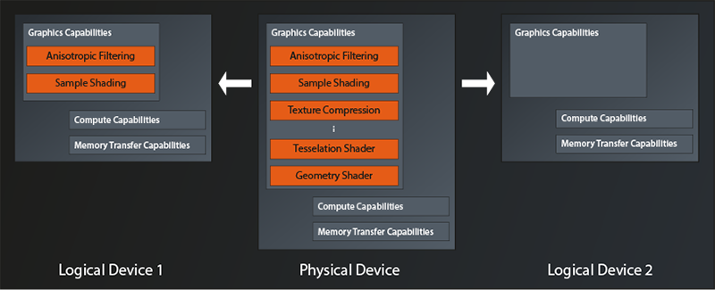
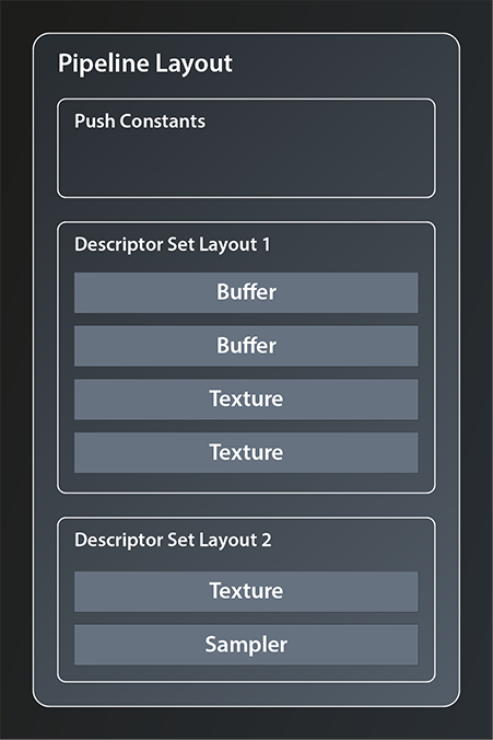
To explain that we need to first talk about descriptors. The Vulkan pipeline and it’s shaders do not access data resources (like e.g. images and buffers) directly. Instead descriptors are used as proxy objects. This indirection allows for the pipeline to be created once and then remain unchanged while still being able to work with changing resources. Those descriptors are always grouped in DescriptorSets, you cannot create a descriptor that is not part of such a set.

We’ll get to actually creating DescriptorSets in the next lesson. To create our PipelineLayout however, we don’t need the actual set but only its layout. As said, the PipelineLayout represents the structure of the data the pipeline is going to work with, so we need to give it the structure of the descriptor sets we’re intending to use. This is what the DescriptorSetLayout is for. A PipelineLayout can contain multiple DescriptorSetLayouts, as depicted in the following example:

There is, however, a limitation to the number of descriptor sets that can be bound to one pipeline. This limit is device dependent and can be as low as 4¹.

So let’s see how we can create our layout:

class Device
{
    ...
    UniqueDescriptorSetLayout createDescriptorSetLayoutUnique( const vk::DescriptorSetLayoutCreateInfo&, ... );
    ...
};

Again the familiar pattern. The create info is very simple, it looks like this:

struct DescriptorSetLayoutCreateInfo
{
    ...
    DescriptorSetLayoutCreateInfo& setFlags( vk::DescriptorSetLayoutCreateFlags flags_ );
    DescriptorSetLayoutCreateInfo& setBindings( const container_t< const vk::DescriptorSetLayoutBinding >& bindings_ );
    ...
};

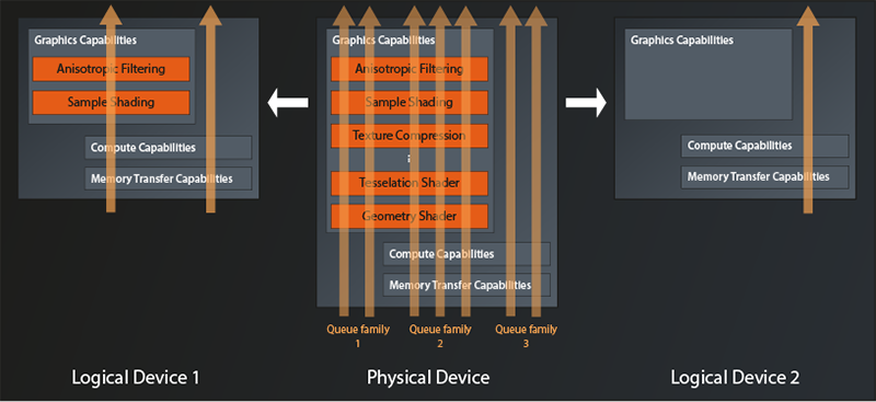
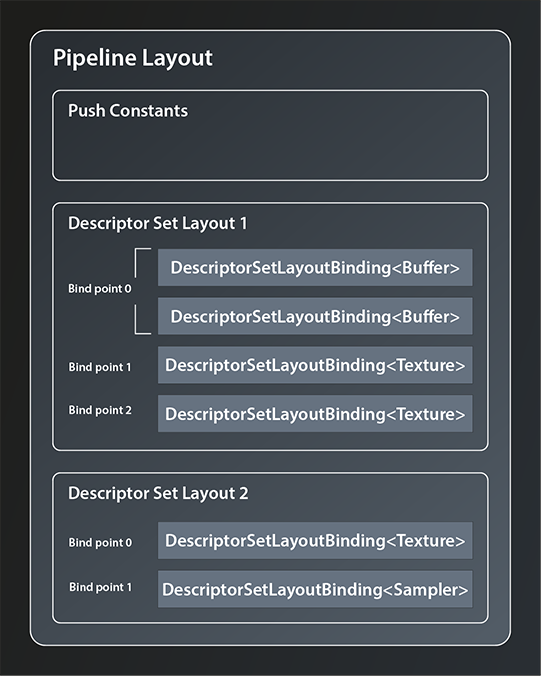
There are a few flags defined but we don’t need any for our use case, so let’s concentrate on the second function. That takes a collection of DescriptorSetLayoutBindings. Those bindings define which concrete types of resources make up the DescriptorSetLayout and in which order. Let me try to illustrate this by refining the example from before:

DescriptorSetLayoutBinding offers the following interface:

struct DescriptorSetLayoutBinding
{
    ...
    DescriptorSetLayoutBinding& setBinding( uint32_t binding_ );
    DescriptorSetLayoutBinding& setDescriptorType( vk::DescriptorType descriptorType_ );
    DescriptorSetLayoutBinding& setDescriptorCount( uint32_t descriptorCount_ );
    DescriptorSetLayoutBinding& setStageFlags( vk::ShaderStageFlags stageFlags_ );
    DescriptorSetLayoutBinding& setImmutableSamplers( const container_t<const vk::Sampler>& immutableSamplers_ );
    ...
};

• the first parameter, the binding_, defines the so-called bind point of this descriptor. You can think of the bind point as the index of the slot in the descriptor set that this resource occupies (see also the image above).
• descriptorType is straightforward as it simply identifies the resource type this descriptor is representing. There are quite a few possible resource types available, in our case eStorageBuffer is the right one to use because both our input and output data are just that: storage buffers.
• you can actually bind multiple descriptors of the same type to one bind point, which is what the descriptorCount_ parameter is for.
• the stageFlags_ define which shader stages are allowed to access the descriptor(s). Since we only have the compute stage, we’ll just pass the eCompute flag.
• finally, we can ignore the immutableSamplers_ parameter for now because we do not have a sampler resource.

So, with that information we can create the bindings for our input and output buffer and feed them into the create info from which we create the DescriptorSetLayout.

vk::UniqueDescriptorSetLayout create_descriptor_set_layout( const vk::Device& logicalDevice )
{
    const auto bindings = std::array< vk::DescriptorSetLayoutBinding, 2 >{
        vk::DescriptorSetLayoutBinding{}
            .setBinding( 0 )
            .setStageFlags( vk::ShaderStageFlagBits::eCompute )
            .setDescriptorType( vk::DescriptorType::eStorageBuffer )
            .setDescriptorCount( 1 ),
        vk::DescriptorSetLayoutBinding{}
            .setBinding( 1 ) 
            .setStageFlags( vk::ShaderStageFlagBits::eCompute )
            .setDescriptorType( vk::DescriptorType::eStorageBuffer )
            .setDescriptorCount( 1 ),
    };
    const auto descriptorSetLayoutCreateInfo = vk::DescriptorSetLayoutCreateInfo{}
        .setBindings( bindings );

    return logicalDevice.createDescriptorSetLayoutUnique( descriptorSetLayoutCreateInfo );
}

So we bind one descriptor representing a storage buffer to binding point one and another one to binding point two.

Completing the Shader Code

Let’s take a quick detour back to our compute shader now. Because we have defined the data layout and told our pipeline the bind points for our data buffers, we can now actually complete the shader code and get rid of the dummy buffers. As said, the shaders access data via the descriptors, so all we need to do now is to tell our shader the bind points of the descriptors that represent the input and output buffer. In GLSL this is done by defining so-called Shader Storage Buffer Objects:

layout( binding = 0 ) readonly buffer inputBufferLayout
{
    uint inputBuffer[];
};

layout( binding = 1 ) writeonly buffer outputBufferLayout
{
    float outputBuffer[];
};

As you can see there is a direct correspondence between the descriptor set layout that we specified above and the layout directives in the shaders. It is essential that the declaration of the bind points for the resources match, otherwise our pipeline won’t work correctly. The readonly and writeonly qualifiers should be self explanatory. You can omit them in which case the resource will be readwrite. Since you can use the same layout declaration syntax for different types of resources, you have to specify the type explicitly. In our case it is buffer. The last identifier is the name of the layout.

You might wonder why it is necessary to declare the actual buffers again in between the parentheses. The answer is that you can structure the buffer into multiple different data blocks as displayed in the following example:

layout( binding = 2 ) buffer MyExampleBuffer
{
  mat4 matrix;
  vec4 vector;
  float lotsOfFloats[];
};

The only requirement is that the size of all fields is known and fixed except for the last one. We don’t need this feature, nevertheless we have to adhere to the syntax and give our buffers a name. Anyway, our shader is now complete and should be fully functional once we’re able to invoke it properly from our pipeline.

Creating the Pipeline

Speaking of the pipeline: with the descriptor set layout defined, we now have all the pieces needed to create it:

vk::UniquePipeline create_compute_pipeline(
    const vk::Device& logicalDevice,
    const vk::DescriptorSetLayout& descriptorSetLayout,
    const vk::ShaderModule& computeShader
)
{
    const auto pipelineLayoutCreateInfo = vk::PipelineLayoutCreateInfo{}
        .setSetLayouts( descriptorSetLayout );
    const auto pipelineLayout = logicalDevice.createPipelineLayoutUnique( pipelineLayoutCreateInfo );

    const auto pipelineCreateInfo = vk::ComputePipelineCreateInfo{}
        .setStage( 
            vk::PipelineShaderStageCreateInfo{}
                .setStage( vk::ShaderStageFlagBits::eCompute )
                .setPName( "main" )
                .setModule( computeShader )
        )
        .setLayout( *pipelineLayout );

    return logicalDevice.createComputePipelineUnique( vk::PipelineCache{}, pipelineCreateInfo ).value;
}

int main()
{
    try
    {
        ...
        const auto descriptorSetLayout = create_descriptor_set_layout( *logicalDevice );
        const auto pipeline = create_compute_pipeline( *logicalDevice, *descriptorSetLayout, *computeShader );
    }
    ...
}

Wohoa, we’ve created our compute pipeline. It has the compute shader and also knows the descriptor layout for our input and output buffers so that it can pass those on to the shader.

There are still a few things missing though. For one, the pipeline knows the layout of the descriptor sets but we didn’t actually create any descriptor set yet. Second, it still needs to be told what to do with all that². That’s what we’re going to cover in the next chapter.

---

1. See https://vulkan.gpuinfo.org/displaydevicelimit.php?name=maxBoundDescriptorSets&platform=windows
2. This might seem a bit stupid – the pipeline should execute the shaders on the input data of course. Well, that might be obvious for you in this simple case. But Vulkan is designed to handle much more complex scenarios. Therefore we need to tell it exactly what we want

Further Reading

• https://vkguide.dev/docs/chapter-4/descriptors/
• https://www.khronos.org/opengl/wiki/Shader_Storage_Buffer_Object

Version 1.0, updated 2022-01-27

Shaders are small programs that are executed on the GPU hardware, usually a lot of them in parallel. Vulkan and OpenGL shaders are written in a language called GLSL (GL Shading Language)¹, which is very similar to C. The shaders are compiled and uploaded to the graphics hardware every time the Vulkan application runs. There are multiple types of shaders that allow you to customize the graphics pipeline at different points, e.g. vertex-, fragment- or geometry shaders. For our compute pipeline however there is only one relevant type, which is the compute shader.

GLSL basics

The most basic shader we can write in GLSL looks something like this:

#version 450

void main() 
{
    
}

To C and C++ programmers this looks pretty familiar, right? The first line, starting with a hash, is indeed called a preprocessor directive just like in C and C++. Every shader should start with this version identifier that denotes the GLSL language version the shader is written in. This allows the compiler to process the code in the best possible way and do detailed checks according to the denoted version.

Most of the other preprocessor directives will be intuitive for C and c++ programmers: #define, #undef, #ifdef, #pragma, #error etc. There are also a few that are specific to GLSL, like #version, but ultimately there’s nothing new here.

The main function is slightly different compared to it’s C/C++ counterparts in that it doesn’t have a return value. Shaders do not return values. But otherwise functions are declared and used in the same way as in C/C++.

Compiling the shader

Another difference between Vulkan and OpenGL is that Vulkan requires us to precompile the shaders. In OpenGL the GLSL code is loaded by the application and then compiled and linked into a program explicitly. Since all of that happens at runtime, the respective driver on the user’s device needs to do all the required heavylifting. This makes OpenGL drivers even more complex than they need to be anyway and may lead to subtle differences in behaviour or even bugs because of the different compiler implementations.

In Vulkan, the GLSL code has to be precompiled into an intermediate binary representation called SPIR-V before loading it into the application and handing it over to the runtime. So instead of raw GLSL the shaders are shipped with the application as SPIR-V bytecode. Compiling SPIR-V to the native binary code for the GPU is much less complex, the drivers can thus be simpler and the potential for bugs and divergences is reduced quite significantly.

The GLSL to SPIR-V compiler that comes with the Vulkan SDK is located in its bin folder and is called glslc. It’s basic usage is very straightforward:

> glslc  <glsl_shader_filename>  -o <compiled_shader_filename>

So let’s compile our minimal shader from above. Create a folder shaders in the project root. In that folder create a text file named compute.comp² and paste the above code into the file. Then create another folder shaders in the build\bin directory and finally run this command³:

> glslc shaders/compute.comp -o build/bin/shaders/compute.spv

That command should terminate without any output (indicating success) and you now should see the file compute.spv in your build/bin/shaders folder.

Nice, we have the shader code in a format now that can be used by Vulkan. However, I don’t want to manually repeat the compilation whenever I change the shader code, so let’s instead add it as a build step to our CMakeLists.txt:

add_custom_target( compute_shader
    COMMAND             "glslc" "${VULKAN_TUTORIAL_PROJECT_ROOT}/shaders/compute.comp" -o "shaders/compute.spv"
    WORKING_DIRECTORY   "${CMAKE_BINARY_DIR}/bin"
)

Now the shader should be compiled every time you build and run the project.

Loading the shader

Okay, we have the precompiled shader now. The next step is to load it into the application and pass it on to Vulkan. The Vulkan C++ representation of a shader is vk::ShaderModule and it is created like this:

class Device
{
    ...
    UniqueShaderModule createShaderModuleUnique( const ShaderModuleCreateInfo& createInfo, ... );
    ...
};

No surprises so far, let’s look at ShaderModuleCreateInfo:

struct ShaderModuleCreateInfo
{
    ...
    ShaderModuleCreateInfo& setFlags( vk::ShaderModuleCreateFlags );
    ShaderModuleCreateInfo& setCode( const vk::container_t< const std::uint32_t >& );
    ...
};

As so often, the flags are just there for future use, which means that we really only have one parameter to set – the shader code in the form of a 32bit uint buffer. Which means that the whole process of creating the ShaderModule is very straightforward:

vk::UniqueShaderModule create_shader_module( 
    const vk::Device& logicalDevice, 
    const std::filesystem::path& path 
)
{
    std::ifstream is{ path, std::ios::binary };
    if ( !is.is_open() )
        throw std::runtime_error( "Could not open file" );

    auto buffer = std::vector< std::uint32_t >{};
    const auto bufferSizeInBytes = std::filesystem::file_size( path );
    buffer.resize( std::filesystem::file_size( path ) / sizeof( std::uint32_t ) );

    is.seekg( 0 );
    is.read( reinterpret_cast< char* >( buffer.data() ), bufferSizeInBytes );

    const auto createInfo = vk::ShaderModuleCreateInfo{}.setCode( buffer );
    return logicalDevice.createShaderModuleUnique( createInfo );
}

The only thing we need to pay a bit of attention to is the mismatch between what the standard library expects when reading data (a pointer to a byte buffer) and what Vulkan expects (a uint32_t buffer). I’ve packaged the shader module creation into it’s own function from the start because it makes the code in main clearer and we’re definitely going to need it more often in the future when we get to the graphics shaders. So with that we can load our compiled compute shader:

const auto computeShader = create_shader_module( *logicalDevice, "./shaders/compute.spv" );

Extending the shader code

The shader we have so far is obviously not useful for anything. Let’s change that. Let’s assume our goal is to multiply each input element by 4.2, which is still not particularly useful, but at least we could demonstrate that the pipeline works and the values are computed. So what we want to do is something like this:

void main()
{
    outputBuffer = inputBuffer * 4.2;   // does not compile
}

That won’t work of course. If you try to compile the shader in that stage, glslc will complain that neither outputBuffer nor inputBuffer are declared. Ultimately we want the buffers to be the GPU buffers we created in the last lesson. But since we don’t know how to do that yet, let’s create some dummy buffers directly in the shader:

int inputBuffer[512];
float outputBuffer[512];

That solves the issue with the undeclared variables, but now we have a new problem. Just like in C++ it is not possible to just multiply a buffer by a factor. And even if it were possible – the whole point of our compute pipeline is to parallelize the calculation by running the shader many times in parallel. So we don’t want the shader code to process the whole buffer, we want each shader instance to only process one element in that buffer. Something along these lines:

void main()
{
    outputBuffer[processingIndex] = inputBuffer[processingIndex] * 4.2;
}

So we need the processingIndex, i.e. the index of the data element that the specific shader invocation is supposed to process. To be able to set this in a meaningful way, we have to take a quick detour and look into how graphics hardware is organized and how Vulkan models compute shader invocations to make use of that hardware.

As mentioned before in this tutorial, GPUs have hundreds of small general purpose processing cores. They are much simpler than the cores in a modern CPU, but because they are so many they can do parallel computations on big datasets really fast. Those small cores are grouped into larger processing units which share registers, caches, scheduler etc and can run multiple batches of work in a hyperthreaded way.

The two main concepts in Vulkan to organize this massive parallelization are the so-called local and global workgroups. Local workgroups are defined in the shader code itself and thus cannot be modified at runtime. A local workgroup essentially defines how many instances of the shader are to be executed simultaneously. In the simplest case the workgroup size is just a one-dimensional number, but Vulkan also allows you to specify two- and three-dimensional workgroups⁴.

Global workgroups (aka Dispatches) on the other hand are created by the host application at runtime. A global workgroup defines how many local workgroups are to be run in parallel. You might wonder why that differentiation was made instead of just having one type of workgroup that directly specifies the number of parallel computations. The reason is that this two-level hierarchy is much better tailored to the architecture of the GPUs, as the driver can better distribute the local workgroups to the available processing units. In addition, the shader invocations in one local workgroup can access workgroup-local memory and share state and data (something we won’t go into further detail here).

We’ll talk more about dispatching the global workgroups in a later episode. For now let’s focus on the local workgroups. As said, those are defined in the shader code by specifying the workgroup layout:

layout( local_size_x = 8, local_size_y = 8, local_size_z = 4 ) in;

This is an example of a three-dimensional local workgroup. In our current usecase the multiple dimensions don’t really add any value, so we can go with a one-dimensional one:

layout( local_size_x = 64 ) in;

As you can see, you can omit the y and z dimension if it’s 1. Note that we’re setting the workgroup size to be smaller than the number of elements in our buffer. It is a recommended best practice to keep local workgroups relatively small (<=64) so that they can fit into one processing unit. That means of course that we’ll have to issue eight of them in our dispatch from the application to process all our data.

Now that we have the workgroup size defined, specifying the correct index into our data is actually very straightforward, as GLSL provides the builtin variables gl_WorkGroupID, gl_WorkGroupSize and gl_LocalInvocationID:

void main()
{
    uint processingIndex = gl_WorkGroupID.x * gl_WorkGroupSize.x + gl_LocalInvocationID.x;
    outputBuffer[processingIndex] = inputBuffer[processingIndex] * 4.2;
}

gl_WorkGroupID is the index of the current workgroup in the dispatch and gl_LocalInvocationID is the index of the shader invocation within this workgroup. The size of a local workgroup can be obtained with gl_WorkGroupSize. All three variables are 3-dimensional vectors, just as the workgroup can be 3-dimensional. So obviously we’d need to also take the y and z values into account if our workgroups had more than one dimension.

So far so good. Our shader is still not doing anything useful, because it isn’t connected to actual input and output buffers yet. Before we can modify it accordingly though we need to understand a bit more about how the compute pipeline works. We’ll therefore leave it as is for the moment and start working on the pipeline next time.

---

1. The GLSL Vulkan profile differs slightly from the one for OpenGL, mostly in that it removes deprecations. Some OpenGL shaders therefore might not compile directly for Vulkan without modifications. However, those modifications should usually be pretty minor.
2. There is no official standard that specifies the extension of .glsl shaders. However, the extensions `.vert`, `.frag` and `.comp` are very common for vertex, fragment and compute shaders respectively. They are also recognized by most tools that work with GLSL (e.g. VS code extensions).
3. Installing the Vulkan SDK should have put its `bin` directory in your path so that the executable is found automatically. If that is not the case you should add that directory to your path by hand and try again.
4. To my knowledge this is pure convenience for when you have to deal with two- and three-dimensional datasets (plus maybe a bit of heritage from graphics programming). I.e. there is no practical difference on the hardware between a one-dimensional workgroup with 256 parallel invocations, and a three-dimensional one with a size of 8x8x4.

Further Reading:

• https://stackoverflow.com/questions/54750009/compute-shader-and-workgroup

Version 1.1, updated 2022-01-23

So, we’re now finally at a point where we can start implementing our first Vulkan pipeline. As said, it’s going to be a compute pipeline because that is the shorter and more straightforward route to doing something meaningful with Vulkan. But rest assured, the graphics stuff will follow after.

A compute pipeline is conceptually very simple: the data ‚flows‘ from the pipeline input through exactly one shader stage (the compute shader) to the output. The key advantage of such a pipeline compared to a classic CPU is its massive parallelization capacity. The GPU can run hundreds of incarnations of the shader kernel at the same time on its processing units, each one usually working with one element of the input data.

We’ll implement a ‚one-shot‘ calculation, i.e. we will copy one block of input data to the GPU, let the pipeline process the data and copy the result back to our main memory, as shown in the following picture:

That doesn’t look too complicated, right? How about we just get started?

Creating the host buffers

As said, we first need a buffer in main memory that holds the data we want to process. In C++ the default data structure for such a buffer is either an array or a vector, depending on whether we know the size at compile time or not. In our case an array seems appropriate for now.

constexpr size_t numElements = 500;
auto inputData = std::array< int, numElements >{};
int counter = 0;
std::generate( inputData.begin(), inputData.end(), [&counter]() { return counter++; } );

As you can see I’ve initialized the input data with ascending integers starting at 0. And while we’re at it let’s also create the buffer that will receive the processed data:

auto outputData = std::array< float, numElements >{};

No need to initialize anything here, we’ll overwrite the data anyway.

Creating the GPU buffers

So, we now have our buffers allocated in main memory. Next thing we need are corresponding buffers in GPU memory that we can transfer our data to and from. Luckily it turns out that you can create something called Buffer from the Vulkan Device, which sounds exactly like what we need:

class Device
{
    ...
    UniqueBuffer createBufferUnique( const vk::BufferCreateInfo&, ... );
    ...
};

There is also the non-unique version, but as mentioned in lesson 2 we’ll use the unique wrappers wherever possible. Let’s have a look at the BufferCreateInfo structure:

struct BufferCreateInfo
{
    ...
    BufferCreateInfo& setFlags( BufferCreateFlags flags_ );
    BufferCreateInfo& setSize( DeviceSize size_ );
    BufferCreateInfo& setUsage( BufferUsageFlags usage_ );
    BufferCreateInfo& setSharingMode( SharingMode sharingMode_ );
    BufferCreateInfo& setQueueFamilyIndices( const container_t< const uint32_t >& queueFamilyIndices_ );
    ...
};

For a change the BufferCreateFlags are actually used and not only reserved for the future. However, we don’t need to define any special creation flags for now, so we can still ignore them.

setSize should be self-explanatory, it’s the size of the buffer in bytes.

The BufferUsageFlags are a bit overwhelming at first because of the sheer number of flags. But for simple data buffers like ours we just need to set vk::BufferUsageFlagBits::eStorageBuffer .

The sharing mode is either vk::SharingMode::eExclusive, which means only one queue will ever access the buffer at the same time. Or it is vk::SharingMode::eConcurrent which means this buffer might be accessed by multiple queues simultaneously. We have only one queue, so we’ll use the exclusive mode.
Setting the queueFamilyIndices is only necessary if the sharing mode is concurrent, so we can ignore that too.

Which means we can create the gpu buffers like this:

const auto inputBufferCreateInfo = vk::BufferCreateInfo{}
    .setSize( sizeof( inputData ) )
    .setUsage( vk::BufferUsageFlagBits::eStorageBuffer )
    .setSharingMode( vk::SharingMode::eExclusive );

auto inputBuffer = logicalDevice->createBufferUnique( inputBufferCreateInfo );

We now could copy that code to create the output buffer, but that would be an unnecessary duplication I’d say. Let’s instead package it into a utility function.

vk::UniqueBuffer create_gpu_buffer( const vk::Device& logicalDevice, std::uint32_t size )
{
    const auto bufferCreateInfo = vk::BufferCreateInfo{}
        .setSize( size )
        .setUsage( vk::BufferUsageFlagBits::eStorageBuffer )
        .setSharingMode( vk::SharingMode::eExclusive );
    
    return logicalDevice.createBufferUnique( bufferCreateInfo );
}

… and call that twice for our input and output buffers:

const auto inputBuffer = create_gpu_buffer( *logicalDevice, sizeof( inputData ) );
const auto outputBuffer = create_gpu_buffer( *logicalDevice, sizeof( outputData ) );

Cool, we have the GPU buffers, now we would like to copy our input data from main memory to the GPU buffer. How do we do that?

The standard way to copy blocks of raw memory in C++ is still the old memcpy function, if we had a pointer to the GPU memory we could use that. But how would we obtain such a pointer?

Well, a bit of searching yields a function that somehow seems to do what we want:

class Device
{
    ...
    void* mapMemory( DeviceMemory memory, DeviceSize offset, DeviceSize size, ... ) const;
    ...
};

The documentation for the corresponding C-function says this function is used to „Map a memory object into application address space“ and it’s result is a „host-accessible pointer to the beginning of the mapped range“. So we should be able to use this pointer as the destination for memcpy.

Sounds great, and the parameters offset and size are self-explanatory enough. But what is the DeviceMemory? We have a Buffer, is that the same? Probably not, otherwise it wouldn’t be two types. But what is it then?

Allocating device memory

The answer is that Vulkan separates the management of the actual memory from its semantic meaning, i.e. from how it is used. This separation enables optimization techniques like allocating a big block of memory and updating it as a whole, but actually using different parts of it for different resources.

So actually our diagram from above becomes a bit more accurate if we modify it like this:

Long story short: we need to explicitly allocate the memory and then attach it to the buffer. The way to do the allocation is with the following function:

class Device
{
    ...
    DeviceMemory allocateMemory( const MemoryAllocateInfo& allocateInfo_, ... );
    ...
};

and the MemoryAllocateInfo interface looks like this:

struct MemoryAllocateInfo
{
    ...
    MemoryAllocateInfo& setAllocationSize( vk::DeviceSize allocationSize_ );
    MemoryAllocateInfo& setMemoryTypeIndex( uint32_t memoryTypeIndex_ );
    ...
};

So we need the allocation size – fair enough, that was to be expected. But now what the heck is the memory type index? I mean, we just want to allocate a block of memory, how complicated can that be?

Now, GPU memory management in Vulkan is indeed a bit more involved than the memory model we’re used to, and the reason is – as so often – enabling performance optimizations. Higher level APIs such as OpenGL or DirectX 11 take care of managing device memory under the hood, but this comes at a cost: the driver implementation basically has to guess how an application intends to use its resources. Will it create another fifty texture images just like the one it just did? Will that big block of memory be accessed from the host over and over again or will the data just sit there and be read by the GPU? Is the application going to destroy resources explicitly once they are not used anymore? It is obviously impossible for a driver to always guess correctly. Chances are therefore that the performance of many applications will not be as good as it could.

Vulkan on the other hand requires us to manage device memory ourselves and be explicit about how we want to use it. For that purpose it introduces the concepts of memory heaps and memory types. Memory heaps are representations of the actual physical types of memory available (e.g. the GPU V-Ram or the host’s main memory), whereas memory types are a virtual construct on top that describes how the respective memory can be used (some details to follow below).

So, to be able to determine the memory type index we need, we first need a list of available memory types and their properties. This we can obtain with the following function:

class PhysicalDevice
{
    ...
    PhysicalDeviceMemoryProperties getMemoryProperties();
    ...
};

And the returned structure looks like this:

struct PhysicalDeviceMemoryProperties
{
    ...
    uint32_t memoryTypeCount;
    container_t< MemoryType > memoryTypes;
    uint32_t memoryHeapCount;
    containter_t< MemoryHeap > memoryHeaps;
    ...
};

As we can see it contains a list of the available memory types. The index we are looking for is an index into that container. The structure also contains a list of the available memory heaps, but since each memory type references its corresponding heap we don’t need to care about those.

The MemoryType struct looks like this:

struct MemoryType
{
    ...
    MemoryPropertyFlags propertyFlags;
    uint32_t heapIndex;
    ...
};

As you probably guessed, the propertyFlags denote the properties of the respective memory type. I won’t go into the meaning of all flags here, at this point only the first three are relevant for us:

• eDeviceLocal means that the memory is physically connected to the GPU
• eHostVisible means that the host can access the memory directly
• eHostCoherent means that host and device always ’see‘ the memory in the same state, i.e. there are no pending cache flushes etc from either side.

As said before, the heapIndex denotes the heap this memory type is based off.

That is all well and good, but we still have no clue how to select the correct memory type. Luckily the logical device knows which requirements our buffer has on the memory it is willing to work with:

class Device
{
    ...
    vk::MemoryRequirements getBufferMemoryRequirements( vk::Buffer, ... );
    ...
};

The MemoryRequirements struct looks like this:

struct MemoryRequirements
{
    ...

    vk::DeviceSize size;
    vk::DeviceSize alignment;
    uint32_t memoryTypeBits;
    ...
};

size should be self-explanatory. The alignment requirements become relevant when the memory is assigned to a resource, we’ll ignore them for now.

The most interesting field for us right now is the memoryTypeBits. This one is telling us is which memory indices are acceptable from the buffer’s perspective. It’s a bitfield, i.e. if the memory type at index 0 is suitable, the rightmost bit (the „1 bit“) of memoryTypBits will be set. If the type at index 1 is suitable, the next bit (the „2 bit“) will be set and so on. Here’s an example illustration where memory types 0 and 2 do meet the memory requirements.

That means we can cycle through the list of available memory types and see which ones are suitable for our input buffer like so:

const auto memoryRequirements = logicalDevice->getBufferMemoryRequirements( *inputBuffer );
const auto memoryProperties = physicalDevice.getMemoryProperties();
for( 
    std::uint32_t memoryType = 1, i = 0; 
    i < memoryProperties.memoryTypeCount;
    ++i, memoryType <<= 1 
)
{
    if( ( memoryRequirements.memoryTypeBits & memoryType ) > 0 )
    {
        // found a suitable memory type
    }
}

But wait, it seems there might be multiple memory types that fit the buffer requirements. Otherwise the structure wouldn’t need a bitmask, a simple index would do. But if we still have more than one possible memory type, which one do we select?

Well, the buffer is not the only one that has requirements on the memory. We ourselves have requirements, too. We want to copy data to that memory from our main memory and this is not possible for all types of GPU memory. In terms of the MemoryPropertyFlags described above that means that we want the memory to be eHostVisible and eHostCoherent. So let’s add our requirements to the selection of the memory index:

const auto memoryRequirements = logicalDevice->getBufferMemoryRequirements( *inputBuffer );
const auto memoryProperties = physicalDevice.getMemoryProperties();
const auto requiredMemoryFlags = vk::MemoryPropertyFlagBits::eHostVisible| vk::MemoryPropertyFlagBits::eHostCoherent;
for( 
    std::uint32_t memoryType = 1, i = 0; 
    i < memoryProperties.memoryTypeCount; 
    ++i, memoryType <<= 1 
)
{
    if( 
        ( memoryRequirements.memoryTypeBits & memoryType ) > 0 &&
        ( ( memoryProperties.memoryTypes[i].propertyFlags & requiredMemoryFlags ) == requiredMemoryFlags )
    )
    {
        // found a suitable memory type
    }
}

So we in principle do have the correct memory index right now, only that the code does look a bit messier than I’d like it to. I’ll therefore refactor the index retrieval into a utility function:

std::uint32_t find_suitable_memory_index(
    const vk::PhysicalDeviceMemoryProperties& memoryProperties,
    std::uint32_t allowedTypesMask,
    vk::MemoryPropertyFlags requiredMemoryFlags
)
{
    for( 
        std::uint32_t memoryType = 1, i = 0; 
        i < memoryProperties.memoryTypeCount; 
        ++i, memoryType <<= 1 
    )
    {
        if( 
            ( allowedTypesMask & memoryType ) > 0 &&
            ( ( memoryProperties.memoryTypes[i].propertyFlags & requiredMemoryFlags ) == requiredMemoryFlags )
        )
        {
            return i;
        }
    }

    throw std::runtime_error( "could not find suitable gpu memory" );
}

… and call it when we do the memory allocation:

const auto memoryIndex = find_suitable_memory_index( 
    memoryProperties, 
    memoryRequirements.memoryTypeBits, 
    requiredMemoryFlags );

const auto allocateInfo = vk::MemoryAllocateInfo{}
    .setAllocationSize( memoryRequirements.size )
    .setMemoryTypeIndex( memoryIndex );
auto memory = logicalDevice.allocateMemoryUnique( allocateInfo );

Make sure to use the allocation size that is returned in the memory requirements, as that might differ from the size of your data¹.

Mapping GPU memory and binding it to the buffer

With the memory being allocated we can now finally map the memory and copy our data into it:

const auto mappedMemory = logicalDevice->mapMemory( *memory, 0, sizeof( inputData ) );
memcpy( mappedMemory, inputData.data(), sizeof( inputData ) );    
logicalDevice->unmapMemory( *memory );

Note that we can immediately unmap the memory after the copy operation. This is possible because we chose a host coherent memory type.

Nice, but we’re not fully done yet. We do have our data in GPU memory, but unfortunately our buffer doesn’t know about that memory yet. Let’s tell it:

logicalDevice->bindBufferMemory( *inputBuffer, *memory, 0u );

Phew, that was much more work than expected, right? But at last we have our data in GPU memory. We’d now have to do pretty much the same again for the output buffer. However, since we’ll use buffer and memory always together in this tutorial², I’ll instead extend the create_gpu_buffer function and do all the allocation and binding in there:

struct gpu_buffer
{
    vk::UniqueBuffer buffer;
    vk::UniqueDeviceMemory memory;
};

gpu_buffer create_gpu_buffer( 
    const vk::PhysicalDevice& physicalDevice, 
    const vk::Device& logicalDevice, 
    std::uint32_t size
)
{
    const auto bufferCreateInfo = vk::BufferCreateInfo{}
        .setSize( size )
        .setUsage( vk::BufferUsageFlagBits::eStorageBuffer )
        .setSharingMode( vk::SharingMode::eExclusive );
    auto buffer = logicalDevice.createBufferUnique( bufferCreateInfo );

    const auto memoryRequirements = logicalDevice.getBufferMemoryRequirements( *buffer );
    const auto memoryProperties = physicalDevice.getMemoryProperties();
    const auto requiredMemoryFlags = 
        vk::MemoryPropertyFlagBits::eHostVisible | vk::MemoryPropertyFlagBits::eHostCoherent;
    
    const auto memoryIndex = find_suitable_memory_index( 
        memoryProperties, 
        memoryRequirements.memoryTypeBits, 
        requiredMemoryFlags );

    const auto allocateInfo = vk::MemoryAllocateInfo{}
        .setAllocationSize( memoryRequirements.size )
        .setMemoryTypeIndex( memoryIndex );

    auto memory = logicalDevice.allocateMemoryUnique( allocateInfo );
    
    logicalDevice.bindBufferMemory( *buffer, *memory, 0u );

    return { std::move( buffer ), std::move( memory ) };
}

… and that simplifies the code in main to:

...
const auto inputBuffer = create_gpu_buffer( physicalDevice, *logicalDevice, sizeof( inputData ) );
const auto outputBuffer = create_gpu_buffer( physicalDevice, *logicalDevice, sizeof( outputData ) );
        
const auto mappedInputMemory = logicalDevice->mapMemory( *inputBuffer.memory, 0, sizeof( inputData ) );
memcpy( mappedInputMemory, inputData.data(), sizeof( inputData ) );    
logicalDevice->unmapMemory( *inputBuffer.memory );
...

Note that we don’t do any mapping or copying for the output buffer as there is no relevant data in that one yet.

That has been quite a big chunk of work this time. Now that we have our input data in GPU memory we can start to think about what we actually want to do with it, and that’s what we’re going to do in the next lesson.

---

1. e.g. because the driver needs some space to store meta information for the buffer
2. Note that it is considered bad practice to allocate individual chunks of memory for each resource because of the performance impact. We’ll do that here for clarity and to get things working as quickly as possible. Once you’re more familiar with the workings of memory management you should definitely look at fueling many resources from a common buffer.

Further reading:

• https://gpuopen.com/learn/vulkan-device-memory/
• https://developer.nvidia.com/vulkan-memory-management

Version 1.0, updated 2021-12-30

I promised already twice that we’d talk about layers and extensions eventually, and now is the time I deliver on that promise.

Both, layers and extensions are a way to enhance Vulkan’s builtin functionality. The main difference between the two is that layers only modify or enhance behavior that is already present, while extensions do add new functionality. We’ll work with both in the course of this tutorial.

Layers

Layers can be thought of as just what their name suggests: additional levels of functionality that an API call passes before it reaches the actual Vulkan core implementation. Layers do not necessarily modify all function calls, depending on the purpose they may leave some alone. Originally Vulkan supported layers for the entire Vulkan environment (so-called instance layers) as well as individual per-physical-device layers. The latter have been deprecated now because it became apparent that there was no real use case for them.

Speaking of use cases: One major use case for layers is adding debugging support to Vulkan. Since the Vulkan core is so optimized for maximum performance, it only does the checks that are absolutely necessary. That means that you can easily issue a function call to the Vulkan core that seems to work fine, but actually does nothing because of a faulty parameter. Or your application might crash without you having the slightest clue what went wrong. Layers can add diagnostics, logging, profiling and other helpful functionality. And because they have to be explicitly switched on to become active, you can just leave them disabled when you ship your application and get the maximum Vulkan performance in production.

Of course, to be able to activate a layer, one should be able to detect whether it is actually supported on the respective system. Here’s the function that lists all the available layers for the instance:

std::vector< vk::LayerProperties > vk::enumerateInstanceLayerProperties( ... );

As you can see, this function is not a member of vk::instance. That makes sense because we already need to pass in the names of the layers we want to enable when we create the instance. The returned vk::LayerProperties structs have the following properties:

struct LayerProperties
{
    ...
    string_t layerName;  
    string_t description;
    uint32_t specVersion;
    uint32_t implementationVersion;
    ...
};

What I dubbed string_t here is actually a vk::ArrayWrapper1D, a class that extends std::array with some convenience functions for strings. It behaves pretty much like a plain old C-string in many ways, so I think it’s clearer to write it that way. The most important property in LayerProperties is the layerName, as that is what we need to pass to the InstanceCreateInfo to turn the layer on.

Okay, so let’s list all the layers that are available to us:

...
void print_layer_properties( const std::vector< vk::LayerProperties >& layers )
{
    for ( const auto& l : layers )
        std::cout << "    " << l.layerName << "\n";        
    
    std::cout << "\n";
}

vk::UniqueInstance create_instance()
{
    const auto layers = vk::enumerateInstanceLayerProperties();
    std::cout << "Available instance layers: \n";    
    print_layer_properties( layers );
    ...
}
...

When you run the program now you should see something like this as the first output:

Available instance layers:
    VK_LAYER_NV_optimus
    VK_LAYER_LUNARG_api_dump
    VK_LAYER_LUNARG_device_simulation
    VK_LAYER_LUNARG_gfxreconstruct
    VK_LAYER_KHRONOS_synchronization2
    VK_LAYER_KHRONOS_validation
    VK_LAYER_LUNARG_monitor
    VK_LAYER_LUNARG_screenshot
    VK_LAYER_LUNARG_standard_validation

In this example the NVIDIA Optimus layer is available on the system, along with some by the Khronos Group (the industry consortium that created the Vulkan standard) and some by LunarG (the company that maintains the official Vulkan SDK).
So far, so good. We’ll get back to some of those layers in a minute. Let’s look at extensions first (as said, device-specific layers have been deprecated, so we’ll not cover them here).

Extensions

In contrast to layers, extensions can actually add new functionality to Vulkan. Many of those extensions will only become relevant for you once you start exploring more advanced stuff. Still, there is one family of extensions that is widely used and that we will need in this tutorial as well: the Khronos surface extensions. We’ll be talking about surfaces in depth when we get to the graphics stuff. But let me give you a quick intro here:

One of the main design principles for Vulkan is it’s platform-independence. There’s nothing in the Vulkan core that is specific to one platform. Drawing onto a screen on the other hand is extremely platform specific, especially in a windowed context. Obviously the drawing functionality can not go into the Vulkan core, therefore it is realized by platform-specific extensions.

But first things first, let’s now have a look which extensions we actually have available. The pattern is the same as the one for layers:

...
void print_extension_properties( const std::vector< vk::ExtensionProperties >& extensions )
{
    for ( const auto& e : extensions )
        std::cout << "    " << e.extensionName << "\n";

    std::cout << "\n";
}
...
vk::UniqueInstance create_instance()
{
    const auto layers = vk::enumerateInstanceLayerProperties();
    std::cout << "Available instance layers: \n";    
    print_layer_properties( layers );

    const auto instanceExtensions = vk::enumerateInstanceExtensionProperties();
    std::cout << "Available instance extensions: \n";
    print_extension_properties( instanceExtensions );

    ...

If you run now, you’ll hopefully see output along the lines of the following:

Available instance extensions:
    VK_KHR_device_group_creation
    VK_KHR_external_fence_capabilities
    VK_KHR_external_memory_capabilities
    VK_KHR_external_semaphore_capabilities
    VK_KHR_get_physical_device_properties2
    VK_KHR_get_surface_capabilities2
    VK_KHR_surface
    VK_KHR_surface_protected_capabilities
    VK_KHR_win32_surface
    VK_EXT_debug_report
    VK_EXT_debug_utils
    VK_EXT_swapchain_colorspace
    VK_NV_external_memory_capabilities

Et voilà, there they are: VK_KHR_surface, VK_KHR_win32_surface and VK_KHR_surface_protected_capabilities¹.

But wait, we’re not done yet: in contrast to the layers, a specific device can have it’s own set of extensions on top of that. And as if that weren’t enough already, instance layers can also come with extensions. Since we’re currently working with the instance, let’s finish that off first.

As it turns out you can pass the name of a layer to enumerateInstanceExtensionProperties and that’ll give you the extensions for that specific layer. Let’s enhance our print_layer_properties function accordingly²:

void print_layer_properties( const std::vector< vk::LayerProperties >& layers )
{
    for ( const auto& l : layers )
    {
        std::cout << "    " << l.layerName << "\n";
        const auto extensions = vk::enumerateInstanceExtensionProperties( l.layerName.operator std::string() );
        for ( const auto& e : extensions )
            std::cout << "       Extension: " << e.extensionName << "\n";
    }

    std::cout << "\n";
}

Indeed, if you run that version you’ll see that e.g. the Khronos validation layer comes with three extensions.

Now let’s complete our tour by looking at the device specific extensions. For that purpose we extend the print_physical_device_properties function as follows:

void print_physical_device_properties( const vk::PhysicalDevice& device )
{
    const auto props = device.getProperties();
    const auto features = device.getFeatures();

    std::cout <<
        "  " << props.deviceName << ":" <<
        "\n      is discrete GPU: " << ( props.deviceType == vk::PhysicalDeviceType::eDiscreteGpu ? "yes, " : "no, " ) <<
        "\n      has geometry shader: " << ( features.geometryShader ? "yes, " : "no, " ) <<
        "\n      has tesselation shader: " << ( features.tessellationShader ? "yes, " : "no, " ) <<
        "\n      supports anisotropic filtering: " << ( features.samplerAnisotropy ? "yes, " : "no, ") <<
        "\n";

    const auto deviceExtensions = device.enumerateDeviceExtensionProperties();
    std::cout << "\n  Available device extensions: \n";
    print_extension_properties( deviceExtensions );
}

This is probably going to give you a long list of device specific extensions. Most of them will be irrelevant for this tutorial, but it’s good to know how much functionality you could potentially use.

Debugging:

So, now that we know more about layers and extensions, let’s make use of some. As said, one main usecase for layers is debugging, so that’s what we’ll do here as well.

You might remember that we can set a list of instance layers to enable in the InstanceCreateInfo. So let’s do that and enable the Khronos validation layer and the corresponding extensions:

vk::UniqueInstance create_instance()
{
    ...
    const auto layersToEnable = std::vector< const char* >{
        "VK_LAYER_KHRONOS_validation"
    };
    const auto extensionsToEnable = std::vector< const char* >{
        VK_EXT_DEBUG_REPORT_EXTENSION_NAME,
        VK_EXT_DEBUG_UTILS_EXTENSION_NAME,
        VK_EXT_VALIDATION_FEATURES_EXTENSION_NAME };

    const auto instanceCreateInfo = vk::InstanceCreateInfo{}
        .setPApplicationInfo( &appInfo )
        .setPEnabledLayerNames( layersToEnable )
        .setPEnabledExtensionNames( extensionsToEnable );

    return vk::createInstanceUnique( instanceCreateInfo );
}

As you can see, there are constants defined for the names of some extensions (in vulkan_core.h), not for the layers though.

If you build and run the program now you might already see the layer in action, depending on the platform you’re on. The (quite lengthy) error message seems to be complaining about the VK_KHR_portability_subset extension not being enabled. This extension is used on systems where Vulkan is in fact implemented as a wrapper aroud another graphics API. You’ll likely encounter this on apple computers for example, where Vulkan is implemented on top of Apple’s own Metal API.

So it looks like we’ll have to enable this extension, but only if it’s present. Let’s do that by modifying our create_logical_device function a bit:

vk::UniqueDevice create_logical_device( const vk::PhysicalDevice& physicalDevice )
{
    ...
    const auto enabledDeviceExtensions = get_required_device_extensions(
        physicalDevice.enumerateDeviceExtensionProperties()
    );
    const auto deviceCreateInfo = vk::DeviceCreateInfo{}
        .setQueueCreateInfos( queueCreateInfos )
        .setPEnabledExtensionNames( enabledDeviceExtensions );

    return physicalDevice.createDeviceUnique( deviceCreateInfo );
}

… with:

std::vector< const char* > get_required_device_extensions(
    const std::vector< vk::ExtensionProperties >& availableExtensions
)
{
    auto result = std::vector< const char* >{};
    
    static const std::string compatibilityExtensionName = "VK_KHR_portability_subset";    
    const auto it = std::find_if(
        availableExtensions.begin(),
        availableExtensions.end(),
        []( const vk::ExtensionProperties& e )
        {
            return compatibilityExtensionName == e.extensionName;
        }
    );
    
    if ( it != availableExtensions.end() )
        result.push_back( compatibilityExtensionName.c_str() );
    
    return result;
}

If you run the program again now, that validation message should no longer be displayed.

Cool, that’s it for now for layers and extensions. Next time we’ll start to implement our first pipeline.

1. These are the extensions that are present on my Windows system. Obviously you will not have the ...win32... extension on a macos or Linux machine but something platform specific.
2. In case you’re wondering about the l.layerName.operator std::string(): an implicit or explicit cast don’t work here. I’m not entirely sure why that is because obviously there is a casting operator available. But it only works if I create a named std::string variable or call the casting operator explicitly.

Version 1.1 updated 2022-02-22

Logical Devices

So we do have a handle to the physical device that we want to work with. One might think that we could now just start to use it directly. Well, not so fast my friends. Vulkan is designed for maximum performance, and therefore it wants to know upfront how we intend to use the GPU so it can optimize for our use case. For this purpose Vulkan introduces the concept of logical devices.

You can think of a logical device as a kind of virtual GPU that is tailored exactly to what you need for your application. But to be clear: we’re not talking about an additional abstraction level that introduces overhead. It’s just a means that allows Vulkan to configure the physical GPU in the best way possible for your application by only turning on features that are actually going to be used. An example of this is depicted in the following diagram¹:

So we have a physical device here that offers quite a few features like e.g. anisotropic filtering, texture compression, tesselation and geometry shaders, and so on. The application on the left configures its logical device to only use anisotropic filtering and sample shading. All the other features of the physical device are being left switched off. The application on the right on the other hand does not turn on any of the graphics features for its logical device, potentially because it only wants to use the compute capabilities.

Queues and Queue Families

Another concept that becomes relevant when creating a logical device are the so-called queues. They too are a means to optimize hardware utilization and thus performance. Let me try to explain.

The architecture of modern GPUs is tailored to massive parallelization of tasks. They can compute the same little program (the shader, or more generic: the kernel) several hundredfold at the same time. But that means that one work package might not actually utilize all that processing power. Imagine e.g. a game that wants to calculate the game physics on the GPU while at the same time rendering the next frame. It might be that neither of the two tasks actually requires the full processing capacity of the device. If we were only able to issue commands to the device as a whole, those tasks would probably have to be executed sequentially (or require some very complex shader programming) and leave us with reduced performance while the GPU is constantly underutilized.

That’s where the concept of queues comes into play. You can think of a queue as a dedicated processing lane on the physical device that supports one or more specific types of tasks. A Vulkan device will almost always provide more than one of them, organized in so called queue families. Each queue family groups one or more queues of the same type (i.e. with identical capabilities) that are able to execute in parallel.

So, when creating the logical device, you also need to specify how many queues of which type (i.e. of which queue family) you intend to use. We can visualize this by extending the diagram above as follows:

The physical device in this example exposes three queue families. One that only supports graphics operations, one which additionally offers compute and memory transfer operations, and one which only supports the latter two. A maximum of two queues can be allocated simultaneously from the first family, three from the second and two again from the third.

The logical device on the left is configured to use one queue from families two and three. Apparently the application wants to parallelize compute tasks with rendering tasks. The logical device on the right only has one queue configured, so the application indeed only intends to use Vulkan for compute operations.

One final note before we actually start implementing: while it is possible to create multiple logical devices from the same physical device, there is no good reason to do so. You won’t get any better parallelization than by using one logical device with multiple queues, it is more work and you loose some options for synchronization and data transfer. Multiple logical devices only make sense when you want to work with multiple physical devices at the same time. But that’s something we won’t go into in this tutorial.

Creating the Logical Device

The logical device is created by the physical device instance:

class PhysicalDevice
{
    ...
    vk::UniqueDevice vk::PhysicalDevice::createDeviceUnique( const vk::DeviceCreateInfo&, ... );
    ...
};

As you can see, in Vulkan the logical devices are just called Device. vk::DeviceCreateInfo provides this (simplified) interface:

struct DeviceCreateInfo
{
    ...
    DeviceCreateInfo& setFlags( DeviceCreateFlags flags_ );
    DeviceCreateInfo& setPEnabledLayerNames( const container_type< const char* const >& layerNames_ );
    DeviceCreateInfo& setPEnabledExtensionNames( const container_type< const char* const >& extensionNames );
    DeviceCreateInfo& setPEnabledFeatures( const PhysicalDeviceFeatures* pEnabledFeatures_ );
    DeviceCreateInfo& setQueueCreateInfos( const container_type< DeviceQueueCreateInfo >& queueCreateInfos_ );
    ...
};

The first property we can set are again some flags. As before, this parameter is reserved for future use, so we can ignore the method.

Next in line are the names of enabled layers and extensions. This looks familiar, right? Didn’t we already have those parameters when we looked at the vk::InstanceCreateInfo?  Indeed, Vulkan distinguishes between instance-level layers and extensions, and device-level layers and extensions². I promise, we’ll get to those very soon, for now let’s ignore them again.

Remember that we were able to query the physical device for it’s features? The next method allows us to selectively enable those features for our logical device. They’re off by default, so in best C++ spirit you don’t pay for what you don’t use in Vulkan. We’re not going to use any features initially, so for now we’ll ignore this parameter as well.

Which leaves the queueCreateInfos_. As described above Vulkan requires us to tell it upfront how many queues of which queue families we intend to use, so that it can configure the physical device optimally. Let’s look at the create info:

struct DeviceQueueCreateInfo
{
    ...
    DeviceQueueCreateInfo& setFlags( DeviceQueueCreateFlags flags_ );
    DeviceQueueCreateInfo& setQueueFamilyIndex( uint32_t queueFamilyIndex_ );
    DeviceQueueCreateInfo& setQueueCount( uint32_t queueCount_ );
    DeviceQueueCreateInfo& setQueuePriorities( const container_type< const float >& queuePriorities_ );
    ...
};

The flags_ parameter is once again reserved for future use (I’ll keep mentioning this to avoid questions – after all, flags usually are something pretty important when configuring a library or similar).

With the next function we can set the index of the queue family we want to create one or more queues from, and with setQueueCount we tell Vulkan how many of those queues we’d like to have available. Via setQueuePriorities you can assign relative priorities to each of the created queues, with 1.0 being the maximum and 0.0 the minimum. This becomes important if the device runs into a situation where it can’t execute all the requested operations at the same time and needs to prioritize.

So with one of these structures we can tell Vulkan to create a number of queues from one family. But what if we wanted to create queues from different families? That’s why DeviceCreateInfo::setQueueCreateInfos accepts a container of these structs, you just create one struct for each family that you need.

Cool, so we could now initialize our DeviceQueueCreateInfo structures and pass them to DeviceCreateInfo. The problem is just: how do we know which queue family index we need to use? To be able to answer this question, we can ask the physical device for information on the queue families it provides:

class PhysicalDevice
{
    ...
    std::vector< QueueFamilyProperties > getQueueFamilyProperties(...) const;
    ...
};

As you might have guessed, this function returns one entry for each available queue family in the vector. QueueFamilyProperties only contains two properties that are of interest to us at the moment:

struct QueueFamilyProperties
{
    ...
    QueueFlags queueFlags;
    uint32_t queueCount;
    ...
};

queueCount gives us the maximum number of queues that you can create from this family. queueFlags is a bitfield (see lesson 2) that tells us which operations this queue supports. The possible flag bits are:

• vk::QueueFlagBits::eGraphics: the queue supports graphics operations
• vk::QueueFlagBits::eCompute: the queue supports compute operations
• vk::QueueFlagBits::eTransfer: the queue supports transfer of data between GPU memory and main memory
• vk::QueueFlagBits::eSparseBinding: sparse binding is an advanced feature where resources (e.g. images) do not have to reside in GPU memory completely. We won’t go into this topic in this tutorial.

So we now can get an overview of the queue families and their capabilities:

...

void print_queue_family_properties( const vk::QueueFamilyProperties& props, unsigned index )
{
    std::cout << 
        "\n    Queue Family " << index << ":\n" <<
        "\n        queue count: " << props.queueCount <<
        "\n        supports graphics operations: " << ( props.queueFlags & vk::QueueFlagBits::eGraphics ? "yes" : "no" ) <<
        "\n        supports compute operations: " << ( props.queueFlags & vk::QueueFlagBits::eCompute ? "yes" : "no" ) <<
        "\n        supports transfer operations: " << ( props.queueFlags & vk::QueueFlagBits::eTransfer ? "yes" : "no" ) <<
        "\n        supports sparse binding operations: " << ( props.queueFlags & vk::QueueFlagBits::eSparseBinding ? "yes" : "no" ) <<
        "\n";
}

...

int main()
{
    ...
    const auto queueFamilies = physicalDevice.getQueueFamilyProperties();
    std::cout << "\nAvailable queue families:\n";
    unsigned familyIndex = 0;
    for ( const auto& qf : queueFamilies )
    {
        print_queue_family_properties( qf, familyIndex );
        ++familyIndex;
    }
    ...
}

Compile and run this and you will get output along those lines:

Available queue families:

    Queue Family 0:

        queue count: 1
        supports graphics operations: yes
        supports compute operations: yes
        supports transfer operations: yes
        supports sparse binding operations: no

    Queue Family 1:

        queue count: 1
        supports graphics operations: yes
        supports compute operations: yes
        supports transfer operations: yes
        supports sparse binding operations: no

    Queue Family 2:

        queue count: 1
        supports graphics operations: yes
        supports compute operations: yes
        supports transfer operations: yes
        supports sparse binding operations: no

    Queue Family 3:

        queue count: 1
        supports graphics operations: yes
        supports compute operations: yes
        supports transfer operations: yes
        supports sparse binding operations: no

In this case it seems there are multiple queue families with identical capabilities. This might be due to some internal differences between the queues which cannot be expressed via the Vulkan interface. Another reason might be that queues from the same family can share resources with minimal overhead. So an implementation might expose multiple queue families with the same capabilities if the hardware implementation does not allow for that.

It is also very common for a GPU to have only a few families with different capabilities, each offering multiple queues. So, while in many cases you might get away with simply selecting the first queue, you should not rely on that being the queue family that supports the functionality you need. You might also find that there actually is no single queue family that has everything you need, in this case you’ll have to use different queues for different tasks.

We’ll again keep it relatively simple in this tutorial and just assume that the physical device has a queue family that fulfills all our needs and select that³:

std::uint32_t get_suitable_queue_family( 
    const std::vector< vk::QueueFamilyProperties >& queueFamilies,
    vk::QueueFlags requiredFlags
)
{
    std::uint32_t index = 0;
    for ( const auto& q : queueFamilies )
    {
        if ( ( q.queueFlags & requiredFlags ) == requiredFlags )
            return index;
        ++index;
    }
    throw std::runtime_error( "No suitable queue family found" );
}

And with this helper function in place we can finally fill our QueueCreateInfo structure. We just have to remember that we’re obliged to set the priorities, even if we have just one single queue⁴.

const auto queueFamilyIndex = get_suitable_queue_family(
    queueFamilies,
    vk::QueueFlagBits::eCompute
);
std::cout << "\nSelected queue family index: " << queueFamilyIndex << "\n";

const auto queuePriority = 1.f;
const auto queueCreateInfos = std::vector< vk::DeviceQueueCreateInfo >{
    vk::DeviceQueueCreateInfo{}
        .setQueueFamilyIndex( queueFamilyIndex )
        .setQueueCount( 1 )
        .setQueuePriorities( queuePriority )
};

I can hear you shouting at me now because I asked for a compute queue, not a graphics one. Yes, I know, most of you are reading this tutorial because they want to do graphics programming. And I promise, we’ll get to that eventually. But setting up a graphics pipeline in Vulkan is a pretty complex task, so there’s quite a way to go still. I therefore think it is better to focus on the simpler problem of getting compute pipeline running first. That will already teach us a lot of the concepts and fundamentals that we’ll need in in any case. That way we can see some success and then build on what we’ve learned to get the graphics working.

Anyway: now that we have our queueCreateInfos, we’re finally able to create our logical device.

const auto deviceCreateInfo = vk::DeviceCreateInfo{}
    .setQueueCreateInfos( queueCreateInfos );

const auto logicalDevice = physicalDevice.createDeviceUnique( deviceCreateInfo );

Compile and run to make sure everything works. Then, as before, let’s wrap all the logical device creation in a function to keep main nice and clean:

vk::UniqueDevice create_logical_device( const vk::PhysicalDevice& physicalDevice )
{
    ...
    return physicalDevice.createDeviceUnique( deviceCreateInfo );
}

int main()
{
    ...
    const auto instance = create_instance();
    const auto physicalDevice = create_physical_device( *instance );
    const auto logicalDevice = create_logical_device( physicalDevice );
    ...
}

Okay, that’s it for now. We have our logical device configured and ready to use. Next time we’ll take a small detour and talk about layers and extensions. After that, we’ll start to actually do something with our graphics hardware.

---

1. This visualization shows a conceptual view, it is not a representation of actual GPU hardware architecture.
2. Actually, device-level layers have been deprecated for a while now and are only kept as part of the interface for backwards-compatibility
3. In the original Vulkan tutorial, the available queues are actually queried when selecting the physical device. This is definitely the more robust way to do it, and I recommend considering this approach for any production code. This is a tutorial, so I try to keep things simple by assuming the queues we need are available on the selected device (I actually did not yet encounter a system that supported Vulkan and didn’t have a graphics and a compute queue family)
4. In this case the function expects an ArrayProxyNoTemporaries (see lesson 2), therefore we cannot pass an rvalue to the function.

Version 1.2, updated 2023-01-12

Alright, enough of the foreplay, let’s get our hands dirty with Vulkan.

Vulkan Instance

The first thing we’ll need to do is to connect our application to the Vulkan runtime. That is done by creating a so-called Vulkan instance, which is represented by the class vk::Instance. This object also encapsulates the application-specific state, so it needs to exist as long as the application uses Vulkan. Technically it is possible to have more than one instance object in your application. However, this is not recommended and might cause issues. The only real-world example I can think of where that might make sense is if your application links to a library that uses Vulkan internally as well.

Creating an instance is done by using the function that we’ve already seen as an example in the last chapter:

vk::UniqueInstance vk::createInstanceUnique( const vk::InstanceCreateInfo&, ... )

The function takes a vk::InstanceCreateInfo as its only required parameter, so let’s have a look at how that one is defined:

struct InstanceCreateInfo
{
    ...
    InstanceCreateInfo& setFlags( vk::InstanceCreateFlags flags_ );
    InstanceCreateInfo& setPApplicationInfo( const vk::ApplicationInfo* pApplicationInfo_ );
    InstanceCreateInfo& setPEnabledLayerNames( const container_t<const char* const >& pEnabledLayerNames_ );
    InstanceCreateInfo& setPEnabledExtensionNames( const container_t<const char* const >& pEnabledExtensionNames_ );
    ...
};

So, apparently this struct has four data fields: some flags, the application info, a collection of enabled layers and another one of enabled extensions¹, whatever those might be. Turns out that the flags are actually reserved for future use, so we can just leave them alone. The layers and extensions will get a lesson of their own, for now we will ignore those two as well.

Which leaves the Application Info. I am not completely sure why there is only the C-style function available here, but that’s the way it is, so let’s use it. We’ll need to create an instance of vk::ApplicationInfo. Here’s a simplified version of its interface:

struct ApplicationInfo
{
    ...
    ApplicationInfo& setPApplicationName( const char* pApplicationName_ );
    ApplicationInfo& setApplicationVersion( uint32_t applicationVersion_ );
    ApplicationInfo& setPEngineName( const char* pEngineName_ );
    ApplicationInfo& setEngineVersion( uint32_t engineVersion_ );
    ApplicationInfo& setApiVersion( uint32_t apiVersion_ );
    ...
};

As you can see this structure contains some meta-information about the application that is about to use Vulkan. It is actually optional to set this data, but a well-behaved program should do so. The information enables the driver to identify your application and potentially adjust some parameters accordingly. This will be absolutely irrelevant for the small tutorial app we’re going to write, but AMD and NVIDIA do optimize their drivers for performance of big AAA games. So, it’s a best practice that doesn’t cost us much, therefore lets just adhere to it:

const auto appInfo = vk::ApplicationInfo{}
    .setPApplicationName( "Vulkan C++ Tutorial" )
    .setApplicationVersion( 1u )
    .setPEngineName( "Vulkan C++ Tutorial Engine" )
    .setEngineVersion( 1u )
    .setApiVersion( VK_API_VERSION_1_1 );

What you pass in the first four parameters is completely up to you, only the last one is somewhat predefined by the Vulkan spec: the API version must denote the version of Vulkan that the application is intending to use. We’re using version 1.1, which was released in 2016, i.e roughly at the same time that Vulkan started to become more widespread. Chances are that if you’re able to use Vulkan at all, your driver will at least support Vulkan 1.1.

With the application info in place we can now create our instance:

const auto instanceCreateInfo = vk::InstanceCreateInfo{}
    .setPApplicationInfo( &appInfo );    
const auto instance = vk::createInstanceUnique( instanceCreateInfo );

As described in lesson 2, we don’t have to worry about the destruction of the instance – the UniqueWrapper will take care of that. If you compile and run your program now, it should run through without any error (without any console output too though).

A note for those of you working on MacOS: with Vulkan SDK version 1.3.216 there has been a change that requires you to enable the portability subset extension explicitly. Failing to do so will yield an exception „Incompatible Driver“. We’ll cover extensions in detail in one of the next lessons, but I’ve updated the code in the repository with a patch that allows you to run the app already now. For more information refer to this article

Congratulations, the first step is done, you have successfully connected your application to Vulkan. We can now start to actually work with our GPUs.

I’d like to make two minor improvements before continue: First I’ll wrap all the instance creation code in a utility function:

vk::UniqueInstance create_instance()
{
    ...
    return vk::createInstanceUnique( instanceCreateInfo );
}

Second: since the Vulkan C++ interface can throw exceptions, I’ll wrap all the code in the main function in a try-catch block:

int main()
{
    try
    {
        const auto instance = create_instance();
    }
    catch( const std::exception& e )
    {
        std::cout << "Exception thrown: " << e.what() << "\n";
        return -1;
    }
    return 0;
}

That looks much cleaner to me. And with that refactoring out of the way, let’s move on to the next step: the physical device selection.

Physical Devices

In many computers there will be only one GPU, either in the form of a dedicated graphics card or integrated in the main processor. But it is also very common to have both types in the same system (e.g in Notebooks), while high-end workstations, gaming machines, servers or specialized hardware might come with multiple dedicated graphics cards. The bottom line here is: You shouldn’t make any assumptions about the available devices upfront but rather check what is there on startup and then make a decision. So let’s do that by using the function vk::Instance::enumeratePhysicalDevices. This function is really convenient, as it takes no parameters and just returns a std::vector<vk::PhysicalDevice>, containing one entry for each device in your system that supports Vulkan:

const auto physicalDevices = instance->enumeratePhysicalDevices();
if ( physicalDevices.empty() )
    throw std::runtime_error( "No Vulkan devices found" );

We can now iterate over the devices to get some more information about each of them. vk::PhysicalDevice has a pretty big interface, but here’s the relevant parts for our current goal:

class PhysicalDevice
{
    ...
    PhysicalDeviceProperties getProperties( ... );
    PhysicalDeviceFeatures getFeatures( ... );
    ...
};

The properties mainly contain metadata about the physical device, such as it’s name, vendor and driver version. They also contain a sub-structure called limits which contains information about the supported range of certain parameters, e.g. the maximum dimensions of the framebuffers (think: the maximum size of the images that can be rendered) or the minimum and maximum width of lines that can be drawn (if you render in Wireframe mode).

The device features are a essentially a long list of boolean flags that are set to true if the respective feature is supported by that device. Those features include things like the availability of certain shader types, the supported texture compression algorithms, anisotropic filtering and much more.

To get a better overview about the hardware we have at hand, let’s write a small function that prints out some properties and features of a device:

void print_physical_device_properties( const vk::PhysicalDevice& device )
{
    const auto props = device.getProperties();
    const auto features = device.getFeatures();

    std::cout <<
        "    " << props.deviceName << ":" <<
        "\n      is discrete GPU: " << ( props.deviceType == vk::PhysicalDeviceType::eDiscreteGpu ? "yes, " : "no, " ) <<
        "\n      has geometry shader: " << ( features.geometryShader ? "yes, " : "no, " ) <<
        "\n      has tesselation shader: " << ( features.tessellationShader ? "yes, " : "no, " ) << 
        "\n      supports anisotropic filtering: " << ( features.samplerAnisotropy ? "yes, " : "no, ") <<
        "\n";
}

… and then call it for the device list we just obtained:

std::cout << "Available physical devices:\n";
for ( const auto& d : physicalDevices )
    print_physical_device_properties( d );

There are of course many more properties and features in the respective structs, so feel free to add output for whatever you’re interested in. If you compile and run the program as described here you should see a list of the available graphics hardware on your system, similar to this one:

AMD Radeon Pro 560:
    is discrete GPU: yes, 
    has geometry shader: no, 
    has tesselation shader: yes, 
    supports anisotropic filtering: yes, 
Intel(R) HD Graphics 630:
    is discrete GPU: no, 
    has geometry shader: no, 
    has tesselation shader: yes, 
    supports anisotropic filtering: yes,

Sometimes there will be only one available device, so there isn’t much of a choice: use it or forget about Vulkan. In our case here we have an integrated and a dedicated GPU so we’ll have to select one, either automatically or by asking the user of your application. In many cases you’ll prefer a discrete GPU over the integrated one because those are usually more powerful and support more functionality. If your application requires specific features you obviously also need to make sure that those are supported and choose the device accordingly.

The takeaway here is: it’s impossible to suggest a generic solution for device selection that will work in all cases. Since this is a tutorial, we’ll just use the first discrete GPU that is available, otherwise the first physical device in the list. We’ll be only using standard features, so this should be fine for our purposes²:

vk::PhysicalDevice select_physical_device( const std::vector< vk::PhysicalDevice >& devices )
{
    size_t bestDeviceIndex = 0;
    size_t index = 0;
    for ( const auto& d : devices )
    {
        const auto props = d.getProperties();
        const auto features = d.getFeatures();

        const auto isDiscreteGPU = props.deviceType == vk::PhysicalDeviceType::eDiscreteGpu;
        if ( isDiscreteGPU && bestDeviceIndex == 0 )
            bestDeviceIndex = index;
    
        ++index;
    }
    
    return devices[ bestDeviceIndex ];
}

And of course we have to call it from our main function:

const auto physicalDevice = select_physical_device( physicalDevices );
std::cout << "\nSelected Device: " << physicalDevice.getProperties().deviceName << "\n";

That’s it, the next step is done: we have selected the physical device that we’re going to work with. Our main function is starting to look a bit cluttered again though. So let’s wrap the whole physical device creation in a function, just as we did with the instance:

vk::PhysicalDevice create_physical_device( const vk::Instance& instance )
{
    ...
    return physicalDevice;
}

int main()
{
    try
    {
        const auto instance = create_instance();
        const auto physicalDevices = create_physical_device( *instance );
    }
    ...
}

That’s much better I think. Now that we have the physical device selected we need to configure it in a way so that it suits our application’s needs. This is what we’re going to do in the next episode.

---

1. The `P` in the function names refers to the fact that the containers contain const char* pointers. The corresponding C-style functions are named setPpEnabledLayerNames and setPpEnabledExtensionNames because they take const char* const* as their argument.
2. Yes, I know, I’m doing the loop over the physical devices and all calls to getProperties and getFeatures twice. So I’m duplicating code and work here. In this case I think that’s okay because it improves the clarity of the code: printing information and selecting the device are two different things. You might want to do those things independently from each other, or you may want to change the implementation of either without affecting the other. So they don’t belong in the same function. The performance penalty is also not relevant her, since cout calls are several orders of magnitude slower than everything else. But of course you’re free to modify the implementation if you have other priorities.

Version 1.0, updated 2021-12-10

The Vulkan C++ interface is part of the official SDK you just installed. To use it, all you have to do is #include <vulkan/vulkan.hpp>¹. There is also a dedicated github repository. The structs, classes and functions provided by this header are all just thin wrappers around the actual Vulkan C-API, so in general it should be pretty easy to find your way around the C++ interface. However, I think it’s useful to point out a few concepts and patterns that will make it easier to follow this tutorial.

Namespace

Everything in the Vulkan C++ wrapper is by default located in the namespace vk. This namespace replaces the Vk... prefix of the functions and classes in the Vulkan C-API. So e.g. the C++ equivalent to Vullkan’s vkCreateInstance is vk::createInstance. You can override the default namespace name by defining the preprocessor constant VULKAN_HPP_NAMESPACE to something else before including vulkan.hpp. We’ll not use this feature though and just go with the default in this tutorial.

Error handling and results

The Vulkan C-API uses result-codes for error handling. Most functions return VK_SUCCESS if they complete without errors and an error code otherwise. By default the C++ wrapper converts those error codes into exceptions. Therefore the C++ do not need to use out-parameters and instead can return their result directly. E.g. this Vulkan C function

VkResult vkCreateInstance( 
    const VkInstanceCreateInfo* pCreateInfo, 
    const VkAllocationCallbacks* pAllocator, 
    VkInstance* pInstance );

becomes the following in the C++ wrapper:

vk::Instance createInstance( 
    const InstanceCreateInfo& createInfo, 
    vk::Optional< const AllocationCallbacks > allocator, 
    ... );  // will throw in case of error

The exceptions thrown by Vulkan C++ are of a type that derives from vk::LogicError or vk::SystemError, which themselves derive from std::logic_error and std::system_error respectively, so you can catch all of them as std::exception. The exceptions wrap the original error code converted to a std::error_code.

It is also possible to turn off exceptions by defining VULKAN_HPP_NO_EXCEPTIONS before including the header. In that case, runtime errors will be handled by the macro VULKAN_HPP_ASSERT which defaults to assert as defined in the cassert header. You can override this macro as well to your custom assertion. Again, we’ll stick to the default of using exceptions for error handling in this tutorial.

Some Vulkan functions may return a result that is not really an error, but neither has the function completed successfully. So the C++ wrapper would be wrong in throwing an exception, but it would equally be wrong to just return a result. For those cases the C++ wrapper uses the class ResultValue:

template <typename T>
struct ResultValue
{
    ...
    Result  result;   // Result is a scoped enum that enumerates the Vulkan result codes
    T       value;

    operator T& ();
    operator const T& ()
};

So, you still can use the result as if it was just the plain result type in most cases. However, this class also allows you to check the result code if it really was a full success.

For clarity reasons I’ll simplify the return type to the T type when showing vk function signatures in most cases.

Vulkan constants and flags

There is an vast number of constants and flags defined by Vulkan C-API. The C++ wrapper converts all of those to scoped enumerations, so you’d e.g. use vk::BlendFactor::eOneMinusSrcColor instead of the original Vulkan constant VK_BLEND_FACTOR_ONE_MINUS_SRC_COLOR. That doesn’t save you much typing, but it adds type-safety and a bit of readability (at least imho).

One thing that might confuse you a bit is the fact that there are always two different C++ types for every set of Vulkan flags: one called ...Flags (e.g. BufferCreateFlags) and one called ...FlagBits (e.g. BufferCreateFlagBits). I’ll go into a bit more detail in a second, but the TL;DR is: just use the ...FlagBits as you would use the C flags, even if a function expects the ...Flags type.

Now for the explanation: Vulkan flags are implemented as bitmasks, so you can combine them with the | operator. The scoped enumerations in the C++ interface normally wouldn’t allow that out of the box, which is why the C++ wrapper implements the | and & operators for every set of ...FlagBits.

However, that alone would still limit the usecases as you cannot define operators like |= or &= as freestanding functions. They need to be member functions, but scoped enums cannot have member functions. Therefore the creators of the Vulkan wrapper introduced the ...Flags classes which wrap the corresponding ...FlagBits and offer the full set of operators.

This probably sounds a bit complicated, but for the users of the SDK it adds a lot of convnience as they can use the ...FlagBits just as they’d use plain old bitmasks and still benefit from the advantages of C++ scoped enums.

The C++ wrapper also provides a vk::to_string function for all those scoped enums, so you can easily output their values to the console etc.

RAII

One of the most important patterns to improve the clarity and correctness of C++ code is RAII (Resource Acquisition is Initialization). A good C++ library therefore better support this pattern.Fortunately, the Vulkan C++ wrapper isn’t letting us down here. However, its RAII support is somewhat opt-in as you have to use the right functions and types, so let’s have a closer look at it.

My guess is that this design choice is based on the nature of the Vulkan C API: Vulkan entities are represented by handles there, you can think of them as being conceptually equivalent to unique IDs or pointers. Since the C-API requires you to do the cleanup yourself (and to do it correctly), you’re free to copy those handles around as much as you wish. All that matters is that you release each acquired resource exactly once.

This concept obviously doesn’t play well with RAII where you want the objects to automatically clean up the resources they acquired upon destruction. One potential solution would be to make the C++ types move-only, another one to use some sort of reference counting internally.

The creators of the Vulkan C++ wrapper chose another way. The classes and structs themselves are not releasing their resources automatically. To achieve RAII behaviour you have to wrap them in a template class called vk::UniqueHandle. This class is very similar to std::unique_ptr in both it’s interface and behaviour:

• you call member functions on the wrapped object with the -> operator
• you dereference the handle (i.e. obtain a reference to the wrapped object) using *
• UniqueHandles can be moved but not copied
• when destroyed, UniqueHandles automatically call the correct Vulkan function to free the underlying resources.

In most cases you don’t have to do the wrapping yourself. Instead, the C++ interface offers two versions of every creation function that returns an object which references a Vulkan resource. Here’s an example

struct Device
{
    ...
    // simplified function declarations for clarity
    Buffer createBuffer( const BufferCreateInfo& createInfo );
    UniqueHandle<Buffer> createBufferUnique( const BufferCreateInfo& createInfo );
    ...
};

I’ve simplified the function signatures and return types for more clarity. As you can see the functions are equivalent except that in the second case the returned vk::Buffer is wrapped in a vk::UniqueHandle. This pattern ( create... returns plain C++ object, create...Unique returns the object wrapped in a UniqueHandle) is the same throughout the Vulkan C++ interface.

We’ll use the create...Unique versions exclusively in this tutorial.

Named parameter idiom

The named parameter idiom is an emulation of a language feature that is available in other languages (e.g. Python, Dart, Ruby, … )². It also has quite a few similarities with the classic builder pattern, only that it doesn’t require any additional classes. The basic idea is that instead of initializing all fields of a class/struct directly via constructor arguments, each field is initialized explicitly via a setter function. The trick is that the setters return a reference to the object itself (just like the assignment operators do) and thus can be chained. So you can initialize every struct in the Vulkan C++ wrapper using this pattern:

const auto appInfo = vk::ApplicationInfo{}
    .setPApplicationName( "Vulkan C++ Tutorial" )
    .setApplicationVersion( 1u )
    .setPEngineName( "Vulkan C++ Tutorial Engine" )
    .setEngineVersion( 1u )
    .setApiVersion( VK_API_VERSION_1_1 );

All data members of structs defined by the C++ header are public, so you could also directly manipulate their values. We’re not going to do that though and stick to the setters.

Arrays and containers

The original Vulkan API follows the common C-Pattern for dynamic arrays: they are passed around and stored as a pointer to the first element and an element count. This is usually considered bad-practice in C++ because it’s error-prone. Instead higher-level constructs like std containers are preferred. The Vulkan C++ API is no exception here, it offers the template classes vk::ArrayProxy and vk::ArrayProxyNoTemporaries for that purpose. They may look intimidating at first, but they actually provide a great convenience to you: whenever a function expects a parameter of one of those types, you can pass in a std::array, std::vector or std::initializer_list without any sort of casting or conversion. Even more convenient: you can even pass in a single value. This makes the calling code really straightforward.

AFAIK the only difference between the two classes is that  vk::ArrayProxyNoTemporaries has explicitly deleted all move constructors, i.e. you can’t pass in any temporary objects.

I’ll use the type alias container_t for either of the two in the code examples. My intention is to make it clear that this parameter essentially expects a container of values to be passed in and not a Vulkan object that you need to create explicitly.

Note that the Vulkan C++ API also always offers the C interface for arrays as you can see in the following example:

struct RenderPassBeginInfo
{
    ...
    // function signatures simplified for clarity reasons
    RenderPassBeginInfo& setClearValueCount( uint32_t clearValueCount_ );
    RenderPassBeginInfo& setPClearValues( const ClearValue* pClearValues_ );
    RenderPassBeginInfo& setClearValues( const container_t<const ClearValue>& clearValues_ );
    ...
};

So it’s up to you whether you use the C-style function pair set...Count / setP... or the single C++ function. This is a C++ tutorial, so we’ll be using the C++ API whenever possible.

Dispatching

You will notice quickly that many functions in the C++ wrapper have an argument Dispatch. That always has a default value, so in most cases you can ignore it.  However, I think it’s important to understand what it is for, therefore I’ll try to quickly explain it:

The core Vulkan API is very stable, and so it is feasible to expose it via a static loader library. The Vulkan C++ wrapper in turn can just use those statically linked functions internally. The same is true for some of the most common extensions – they are included in the loader library. However, if you want to use functions from extensions that are not included, you need to find a way to make them accessible. There are basically two options here: you provide a loader library that includes those extension functions as well, or you link to them dynamically.

The C++ wrapper provides maximum flexibility here by giving every function that calls into the Vulkan API the Dispatch argument which allows you to customize the loading. It defaults to using the standard static loader library as described above, and we’ll just leave it at that whenever we can. This is why I’ll also usually omit it when I show function signatures.

Conclusion

You now should have a rough overview about the concepts used by the Vulkan C++ API. As mentioned previously: for clarity reasons I’ll simplify the vk function signatures to the parts that are relevant for us and thus omit some parameters and qualifiers like noexcept in the code examples from now on.

With that being said, I think we’re now prepared to dive into Vulkan for real, which we’ll start doing in the next lesson.

---

1. Note that, while the C++ support comes as a header-only library, you still have to link against the Vulkan binary library to use it.
2. The C++ 20 standard actually does support named parameters (they are called ‚designated inititalizers‘), and the Vulkan C++ interface also can be configured to work with those. We’ll not do that in this tutorial because the standard is pretty new and chances are that many people are not yet on a compiler supporting it fully.

Version 1.0, updated 2021-12-03

Prerequisites

Compiler toolchain:

The code for this tutorial should work with any compiler that supports the C++17 standard. Since you’re looking at tutorial that uses C++ I assume most of you already have such a C++ toolchain working. But if not, here are a few suggestions:

• if you’re on Windows, the Visual Studion Community Edition is probably the most convenient C++ environment to install
• on Mac, Xcode is the default. I’m not really a fan of that IDE, but it does the job. You can easily install it from the AppStore.
• if you’re on Linux or don’t want to use a full-fledged IDE, you might want to look at VS-Code. It’s a pretty awesome editor that runs on multiple platforms. And with a few extensions it can be converted into a veritable C++ development environment.

CMake:

Because we want to develop a cross-platform graphics application, we should make sure that our project can easily be built on multiple platforms. The most widespread way to do that for C++ is to use CMake. Please download and install the latest version for your platform.

Conan:

Conan is a package manager for C++, similar to e.g. Pypi for Phython. Using Conan makes dependency management a lot easier in many cases. Please refer to their setup guide for information on how to install it on your platform.¹

Vulkan SDK

We want to develop a Vulkan application, so it might actually be a good idea to install the official Vulkan SDK. Please go to the LunarG website and download and execute the installer for your platform. The location where you put the SDK is not relevant.

Alright, your environment should be set up now, so let’s get going with our project.

Project setup

Source code checkout

Go to the bitbucket / github repository (see links in the sidebar on the right) and clone it to your computer. Then checkout the branch for lesson_1:

> git checkout lesson_1

Creating the project files

I prefer to have my project files in a separate folder rather than mixed with my source files etc. Therefore I usually create a build folder. Navigate to your project folder and run the following commands on your console:

> mkdir build
> cd build

Next you’ll need to run conan to install the dependencies. In your python environment (if that’s where you installed conan) run:

> conan install ..

This shouldn’t take more than a few seconds, because at this point we don’t have any dependencies (this will change over the course of this tutorial).

Finally we need to run cmake:

> cmake .. -G <your desired project file type>

That’s it, you now should have a project file for your environment in the build folder.2 Open it in your IDE (if that’s what you use) and try to compile and run the project to make sure everything works.

We’re now set up to get started for real. In the next lesson we’ll have a look at some of the basic concepts in the C++ wrapper before we finally get our hands dirty and start programming Vulkan.

---

1. if you’re on mac you might be tempted to install Conan via homebrew. My experiences here haven’t been so good, since brew only offerered an outdated version of Conan which then didn’t work due to a certificate error. Better install as a python package in a virtual environment.
2. CMake should be able to locate the Vulkan SDK automatically. If it doesn’t, please set the CMake variable VULKAN_SDK_ROOT to the path to the Vulkan SDK folder on your machine and try again.

Version 1.0, updated 2021-11-26

About Vulkan:

There is a lot of information out there on what Vulkan is, it’s history and how it compares to other graphics frameworks. I therefore won’t repeat all that here and instead refer you to the various sources on the web^1,2.

So, just as a very brief overview: Vulkan is a 3D graphics and parallel-computing API, similar to DirectX or Metal. Unlike those it is an open standard and designed to be platform-agnostic. It’s main target hardware are GPUs but it is by no means limited to those.

Vulkan differs from it’s older sibling OpenGL in that it is a lower-level abstraction. This means that you have a lot more control over what’s actually happening on the hardware and thus can often achieve higher performance. The price you pay for those advantages is a much more verbose API which you will soon get to know.³

About this tutorial:

You’ll find quite a few tutorials out there on how to get started with Vulkan. However, most of them use its native C-API, others only cover certain aspects or use higer level frameworks. I’m a C++ developer so I would like to be able to use the features that this language has to offer, while still having control and understanding of the fundametal workings. Unfortunately there is relatively little information on the C++ wrapper that comes with the Vulkan SDK. I think that’s a shame because the wrapper is actually pretty good imho. So by writing this tutorial I want to help closing this gap.

You don’t need to have any previous knowledge about Vulkan or any other graphics framework to follow along. However, I won’t go into details about the C++ code itself, so a solid understanding of C++ is recommended. I’ll provide code examples with the most important parts in the text. Additionally there will be a complete, working version of the respective state of the project in the github / bitbucket repositories.

What you’ll need:

The operating system and compiler you use doesn’t really matter for following along. Vulkan should be supported on any reasonably modern computer system with one of the common OSs. I’ll check that my code works on Windows, macos and Linux.
Additionally you’ll need the following tools:

• a C++ compiler toolchain that supports the C++17 standard
• the conan package manager for C++
• CMake.

We’ll cover the system setup process step-by-step in the next chapter

---

1. https://en.wikipedia.org/wiki/Vulkan
2. https://www.vulkan.org/
3. This is actually pretty similar to C++ compared to higher level languages such as python: you gain control and potentially performance at the cost of convenience